What is SVM?

SVM is a supervised classification method that separates data using hyperplanes.

SVM is a supervised machine learning algorithm is a representation of the examples as points in space, mapped so that the examples of the separate categories are divided by a clear gap that is as wide as possible. New examples are then mapped into that same space and predicted to belong to a category based on which side of the gap they fall.

In addition to performing linear classification, SVM’s can efficiently perform a non-linear classification using what is called the kernel trick, implicitly mapping their inputs into high-dimensional features spaces. (Non-Linear data is basically which cannot be separated with a straight line )

How SVM works?

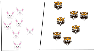
In order to understand how it works, let’s consider a rabbit and tiger example (two data points for visual explanation only). Let’s consider a small scenario now for a second pretend you own a farm. Let’s say you have a problem and want to set up a fence to protect your rabbits against the Tigers.

But, where do you build your fence?

One way to get around a problem is to build a classifier based on the position of the rabbits and tigers. You can classify the group of rabbits as one group and group of tigers as another group

Now, if I try to draw a decision boundary between the rabbits and the tigers it looks like a straight line (please refer below image), now you can clearly build a fence along this line. This is exactly how SVM works, it draws a decision boundary which is a hyperplane between any two classes in order to separate them or classify them.

But, how do you know where to draw a hyperplane?

The basic principle behind SVM is to draw a hyperplane that best separates the two classes, in our case the two classes are the rabbits and the Tigers, so you start off by drawing a random hyperplane and then you check the distance between the hyperplane and the closest data points from each class.

These closest on your data points to the hyperplane are known as support vectors and that’s where the name comes from support vector machine so basically, the hyperplane is drawn based on these support vectors. Normally the hyperplane which has the maximum distance from the support vectors is the most optimum hyperplane and this distance between the hyperplane and the support vectors is known as the margin.

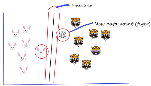
Let’s say if we add a new data point (another tiger added) and now I want to draw a hyperplane to separate the two classes in the best way. So, I start by drawing a hyperplane as shown in the above picture and then I check the distance between the hyperplane and the support vectors and I try to check whether the margin for this hyperplane is maximum or not. In this case, the margin is less.

In the second scenario, I draw a different hyperplane as shown in the picture below and then I check the distance between the hyperplane and the support vectors and I try to check whether the margin for this hyperplane is maximum or not. Margin is high in this case.

Margin is high when compared to this hyperplane with the previous one. Therefore, I choose this hyperplane, as a thumb rule, the distance between the support vectors and the hyperplane (margin) should be maximum. This is how we have to choose the hyperplane.

Our data has been linearly separable as of now, which means you can draw a straight line to separate the two classes. What can we do if we have our datapoints as below? We cannot draw a hyperplane as it doesn’t separate the two classes at all.

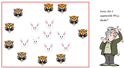
Introduction to Non-Linear SVM

Non-linear SVM is used when the data can’t be separated using a straight line.

We use kernel functions in this case that help transform the data into another dimension that has a clear dividing margin between the two classes. Kernel functions help transform non-linear spaces into linear spaces.

It transforms the two variables x and y into a new feature space involving a new variable called Z. So far, we are plotting our data on two-dimensional space. Now, we are basically doing in three-dimensional space. In 3D space, we can clearly see a dividing margin between the two classes and we can go ahead, and separate the two classes by drawing the best hyperplane between them.

Tuning parameters of SVM

Tuning parameters value for machine learning algorithms effectively improves the model performance. Let’s look at the list of parameters available with SVM. Let’s take a small example,

By considering the length of the post, I do not show the code. Detailed examples with coding will be included in my next blog.

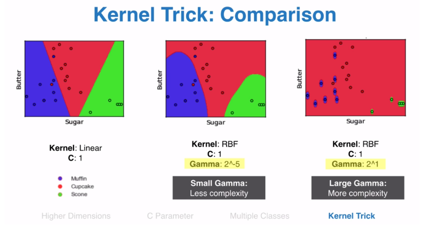
C — It is the regularization parameter. It allowed you to decide how much you want to penalize the misclassified points.

Kernel — It specifies the kernel type to be used. There are different kernel options such as linear, radial basis function (RBF), polynomial and sigmoid. Here “rbf” and “poly” are useful for non-linear hyper-plane.

Gamma — It is the kernel coefficient for the ‘rbf’, ‘poly’ and ‘sigmoid’. Small Gamma gives less complexity and larger gamma gives more complexity.

Pros and Cons — SVM

Pros:

• It is useful for both linearly Separable (hard margin) and Non-linearly Separable (soft margin) data.
• It is effective in high dimensional spaces.
• It is effective in cases where a number of dimensions are greater than the number of samples.
• It uses a subset of training points in the decision function (called support vectors), so it is also memory efficient.

Cons:

• Picking the right kernel and parameters can be computationally intensive.
• It also doesn’t perform very well, when the data set has more noise i.e. target classes are overlapping
• SVM doesn’t directly provide probability estimates, these are calculated using an expensive five-fold cross-validation.

This is a simple visual introduction to SVM’s. Hopefully, this will serve as a good starting point for understanding the Support Vector Machine. I will show how to implement SVM in a SAS Enterprise Miner in my next post with a case study.

Keep learning and stay tuned for more!